Introduction
In version 1.3 of RealBridge we added double-dummy analysis. This isn’t anything new, and we used the standard piece of open-source software – but we did it in a “non-standard” way, and the details might be useful to others.
In particular, this post explains how to run a specific bit of open-source software – the DDS library, written in C – inside a web browser. It will be of particular interest to anyone developing web-based bridge software, but of more general interest to web developers interested in client-side deployment of software written in non-web-native languages such as C or C++.
The Double-Dummy Solver library (DDS)
The DDS library, written by Bo Haglund and Soren Hein (with contributions from others) is a well-optimised open-source double-dummy solver, the purpose of which is to evaluate how good different choices of play are during bridge deals.
A bridge deal has four hands of thirteen cards each, and the four players play as two teams of two, or partnerships. During the play of a deal, one of the players becomes dummy and their hand is placed face-up on the table. The three remaining players can see twenty-six of the cards (their own hand, plus the dummy), and the other twenty-six are hidden.
This partial-information or uncertainty is what makes the game interesting – but it also makes analysing the play extremely challenging. A simpler problem – and one that has the advantage of a definite answer – is what the best play would be if you knew the complete layout of all the cards in advance. This is what “double-dummy” refers to – it’s simply an obscure way of saying “everyone knows the whole hand”.
Under that condition, there’s a single double-dummy result, which is what happens if everyone makes the best choice possible at every turn.
Given a deal, a trump suit and a declarer, the DDS library can efficiently compute the double-dummy result. Moreover, given the current state of play at any point during a deal – and assuming perfect play thereafter – it can tell you the eventual result of each of the legal cards you could play. That is, it can tell you how good each of the choices is at any point.
Play recaps with double-dummy analysis
When reviewing what happened during a game of bridge, players like to be able to check the double-dummy analysis – it can help identify errors, which can help you learn to avoid them in future. Now, not every double-dummy error is actually a mistake – you can make the correct with-the-odds play and lose to an inferior play that happens to work this time. This is part of the fun of the game! With enough luck, anything is possible…
Nevertheless, double-dummy analysis is a useful tool to have in your bag, and it’s much easier to use software that can compute it in a fraction of a second than try to work it out by hand.
DDS as a web service
Existing bridge sites offering double-dummy analysis usually wrap up DDS, or other software with equivalent functionality, as a web service. That is, the client makes a request to a server, the processing happens on the remote server, and then the server sends the results back to the client to display to the user.
This used to be the only way to expose the capabilities of library software to browsers, but it comes with some drawbacks. The main one is the latency of response: given that a DDS solve of a full hand takes around 50 milliseconds, the round-trip latency to the server and back is likely to be a significant fraction of the total time. If the client and server are far apart – for instance, on different continents – the communication latency will far exceed the processing time.
Another disadvantage is that the service provider has to provide a server! There is a potential scaling problem inherent in this – it’s likely that double-dummy queries will be an irregular workload (eg, when lots of players finish sessions at the same time, and then all look through the deals).
There’s another more subtle point about scaling and performance. The DDS solver has some built-in caching of deal-positions and results. When it explores the full “game-tree” of possibilities for a deal, equivalent positions will come up multiple times, and it’s much faster to be able to look up results we’ve already computed than recompute the same thing multiple times.
Now, the library is clever enough to reuse this information across separate queries. If an incoming query comes from the same deal, with the same trump suit, the solver can simply reuse results already in its cache. This means that in the case that several consecutive queries are about the same contract and line-of-play, the later queries will return near-instantly, with no work to do.
This means that if, somehow, each client had its own private version of DDS to use, its queries would be much more efficient – since typical use is to make lots of queries about the same deal consecutively. Whereas if we have one centralised server processing requests for lots of users, it’s much harder to efficiently reuse data without doing significant extra engineering.
All this points towards one thing: what we really want to do is run the DDS library locally, on the client’s machine, separately for each user. While a few years ago this would have been a pipedream, more modern technologies make it pretty straightforward to get the best of both worlds – faster and more efficient for the user, and simpler and easier for the service provider!
Compiling with Emscripten
If we suppose our use case is a webpage or web app, this means we want to run DDS directly in the client’s browser. To do that, we can’t compile the C code to a binary – because the binary will depend on the OS and hardware it’s compiled on (or for). We need something else, something platform-independent that browsers understand. Fortunately, there are standards and software out there that can help us!
Emscripten is a tool for turning C or C++ into JavaScript. More specifically, it’s a compiler toolchain that uses LLVM to compile C/C++ to WebAssembly.
Emscripten itself has been around for a relatively long time – the project started in 2010 – and was a big reason for the standardisation process that created WebAssembly. Because it’s a standard, and supported in all major modern browsers, WebAssembly is now a mature technology.
Once the toolchain is installed, compiling a simple C program with Emscripten is straightforward:
emcc main.c
This will emit two files: a.out.js and a.out.wasm
The WASM file is our code, compiled to WebAssembly – instructions for a virtual machine that browsers know how to execute efficiently. The JavaScript file contains the “glue code” that allows us to interact with the compiled functionality from JS.
We can run our compiled code as a console application via the Node.js runtime. The Emscripten toolchain bundles Node.js with it, so all we need to do is:
node a.out.js
Without any further instructions, Emscripten will simply generate the executable consisting of whatever the C main() function does. The JavaScript glue will then execute this main() functionality and then exit.
This isn’t exactly what we want to achieve – we have library functionality that we want to call on-demand, multiple times. That is, we don’t want the JS module to exit, we want it to stay alive indefinitely. Fortunately, with a bit more work and some handy compiler options we can do this too.
Compiling DDS with a C-function wrapper
We want to call two DDS functions from JavaScript:
- SetResources – function to initialise the system.
- SolveBoardPBN – function to solve a deal or position.
It’s convenient to write a small C-wrapper to translate parameters into the form expected by DDS. Ours looks like this:
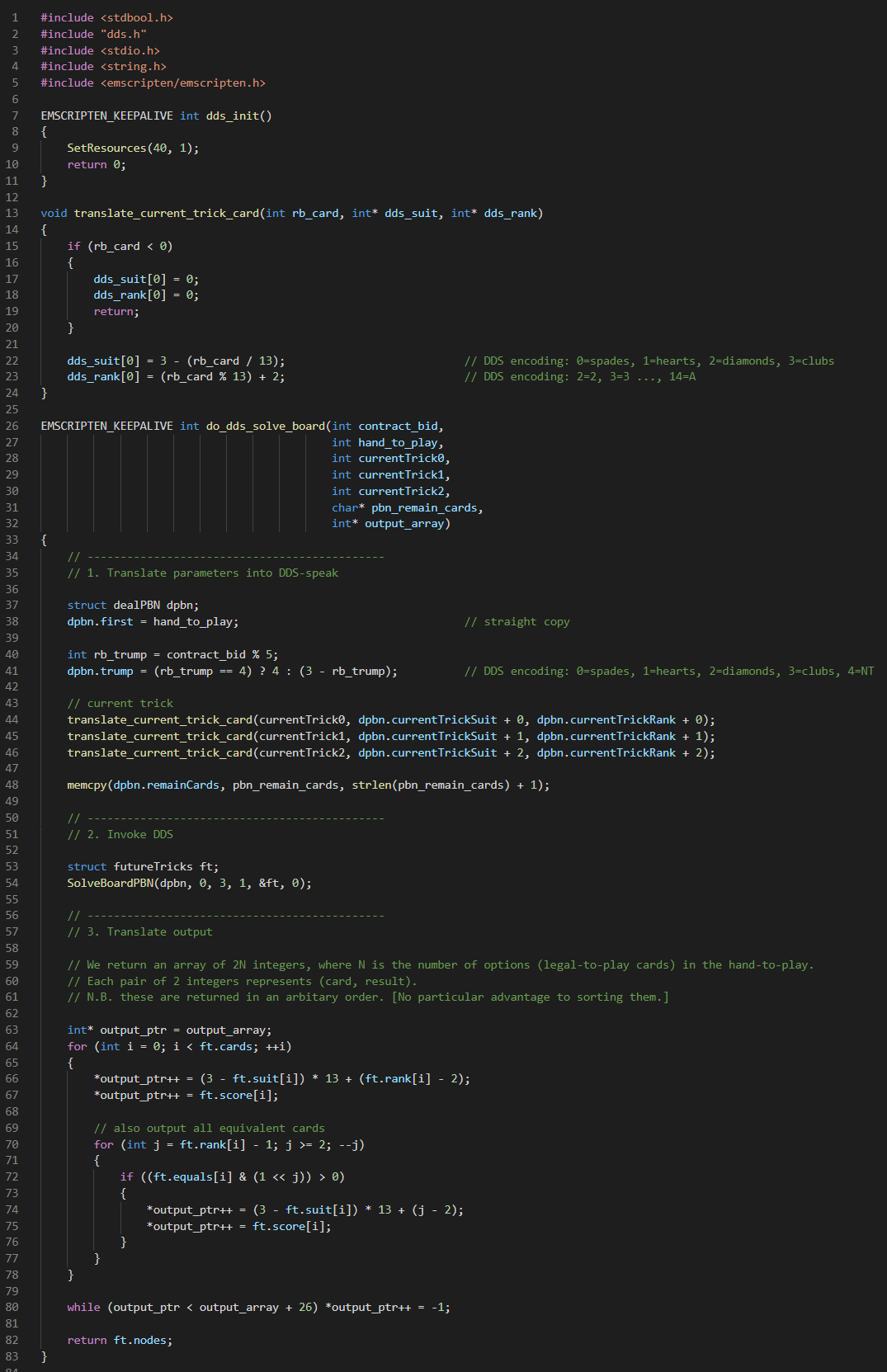
Things to note are:
- We decorate the C functions we want to call from JavaScipt with the EMSCRIPTEN_KEEPALIVE macro (defined in emscripten.h). This tells the compiler not to strip out that function from the compiled output.
- All of the work in the do_dds_solve_board function is simple translation of the input and output data. We write the output into an array of 26 integers, since this is easy to read and write on the JavaScript side.
- We tell the compiler to generate JavaScript that doesn’t run-and-then-exit. We do this by adding -sNO_EXIT_RUNTIME=1 to the command line.
We can now try to compile DDS!
emcc -sNO_EXIT_RUNTIME=1 <dds-source-files> main.c
We get a few compiler errors, so there are a handful of places we need to modify the DDS code to compile with Emscripten:
- There are some string-related functions in Par.cpp that Emscripten complains about. Fortunately, we don’t need any of the functions in Par.cpp for our purposes, so we can simply leave that file out.
- In dds.h, Emscripten is fussy about the declarations of structs containing other structs, so we need to add the word struct a few times.
To actually run the code successfully, we also need to modify the System::GetHardware function. In normal operation, this detects the number of cores and free memory available in the system. The idea is to use all of the resources in the system when solving multiple deals in parallel.
However, we only want to solve one deal at a time, so we can hard-code the GetHardware function to report a single core and 50MB of memory. This will cause DDS to run in single-threaded mode, with one of its “small” threads.
To get this to work, we also need to tell Emscripten to increase the amount of memory available to be allocated (from the default of 16MB):
emcc -sINITIAL_MEMORY=52428800 -sNO_EXIT_RUNTIME=1
  <dds-source-files> main.c
Testing the code from JavaScript
We’ve successfully compiled the code, but can’t do anything useful with it yet – first we need to tell Emscripten which functions we’re going to call from JavaScript:
emcc -sINITIAL_MEMORY=52428800 -sNO_EXIT_RUNTIME=1
  -sEXPORTED_FUNCTIONS="_free,_malloc,_do_dds_solve_board, _dds_init"
  -sEXPORTED_RUNTIME_METHODS="getValue,ccall,allocateUTF8"
  <dds-source-files> main.c
Here, the EXPORTED_FUNCTIONS are the C functions we want to call. Note that each of them gets a leading underscore character when exported. On the other hand, the EXPORTED_RUNTIME_METHODS are JavaScript script functions generated by emcc in the a.out.js file. More specifically, we use getValue to read the 32-bit integers in the generated output array, and we use allocateUTF8 to convert a JavaScript string containing the deal information into a C-style string for input to SolveBoardPBN.
With all of that done, we can write a simple test case to make sure it works:
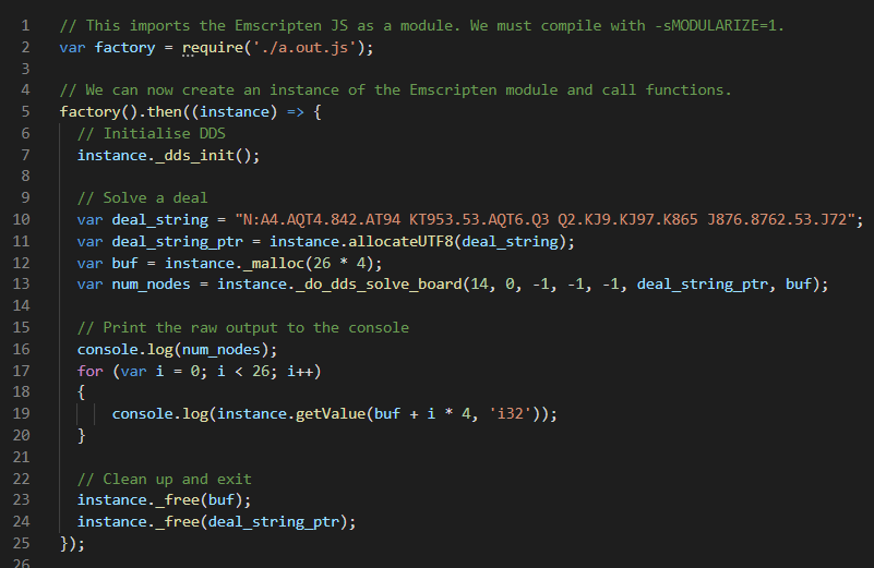
As noted in the comment, to import the Emscripten JavaScript as a module, we need to compile it with -sMODULARIZE=1. This is convenient for this little test, which we can run via Node.js on the command line.
The test does a single double-dummy solve of the given deal, returning 26 integers. Each pair of integers is of the form (card, result): the eventual double-dummy result of playing each possible card.
Running DDS in a WebWorker
A more likely useful scenario is to run DDS inside a webpage. Although it’s fast, the processing for a double-dummy solution isn’t instant, so it would be best to use a separate thread to do the work – that way we don’t cause any hitches on the main processing thread.
Happily, using a WebWorker makes this very simple. Here we have to compile without –sMODULARIZE=1, but then we can use this useful function at the top of our WebWorker:
importScripts("./a.out.js");
(The importScripts function is part of the WebWorker API.)
This defines a variable Module, and we can subsequently call our functions through it, eg:
Module._dds_init()
Of course, the exact details of the WebWorker will depend on the app or webpage it’s communicating with.
Conclusion
Incorporating library functionality into web-based software used to require wrapping software as a web-service and providing servers to run it – but with modern compilation tools and browser capabilities we can now run more types of software directly. This can make developing fully-featured web experiences both quicker and simpler.
 completely before all of the work for sample
  can kick off. (Though there are dynamic-programming-style optimisations available to avoid doing redundant work.)
 with the loading for iteration
  we hide a lot of the memory latency. (And this is enough: unwinding the loop two iterations is slower again.)
 :
:![\[ \vec{\boldsymbol{R}}_1=\frac{1}{4\pi} \oint \vec{\boldsymbol{\omega}}\, R(\vec{\boldsymbol{\omega}}) \, d\Omega \]](https://grahamhazel.com/blog/wp-content/ql-cache/quicklatex.com-5fd295a43d54a696d6d42c98079b9b61_l3.png "Rendered by QuickLaTeX.com")
![\[ \vec{\boldsymbol{n}} \! \cdot \! \vec{\boldsymbol{R}}_1=\frac{1}{4\pi}\oint\vec{\boldsymbol{n}}\!\cdot\!\vec{\boldsymbol{\omega}}\, R(\vec{\boldsymbol{\omega}}) \, d\Omega \]](https://grahamhazel.com/blog/wp-content/ql-cache/quicklatex.com-23560c7778e097787eb2ffddd70e5b60_l3.png "Rendered by QuickLaTeX.com")
![\[ =\frac{1}{4}\left( \frac{1}{\pi} \int_{H+}\vec{\boldsymbol{n}}\!\cdot\!\vec{\boldsymbol{\omega}}\, R(\vec{\boldsymbol{\omega}}) \, d\Omega +\frac{1}{\pi}\int_{H-}\vec{\boldsymbol{n}}\!\cdot\!\vec{\boldsymbol{\omega}}\, R(\vec{\boldsymbol{\omega}}) \, d\Omega \right) \]](https://grahamhazel.com/blog/wp-content/ql-cache/quicklatex.com-f8073d3ab4c779eb128488c89b65b57b_l3.png "Rendered by QuickLaTeX.com")
![\[ \vec{\boldsymbol{n}}\!\cdot\!\vec{\boldsymbol{R}}_1=\frac{1}{4} \left( I(\vec{\boldsymbol{n}}) - I(-\vec{\boldsymbol{n}}) \right) \]](https://grahamhazel.com/blog/wp-content/ql-cache/quicklatex.com-cde775111d716b799794a74087a111e3_l3.png "Rendered by QuickLaTeX.com")
![\[ I(\vec{\boldsymbol{n}})=\frac{1}{\pi}\int_H\vec{\boldsymbol{n}}\!\cdot\!\vec{\boldsymbol{\omega}} R(\vec{\boldsymbol{\omega}}) d\Omega \]](https://grahamhazel.com/blog/wp-content/ql-cache/quicklatex.com-ebe7801370189a61c51cc8bee239d301_l3.png "Rendered by QuickLaTeX.com")
 is the geometry term.
 by
by  and compute the SH coefficients of independently:
![\[ I_0=\frac{1}{\pi}\int_H\vec{\boldsymbol{n}}\!\cdot\!\vec{\boldsymbol{\omega}}\, R_0 \, d\Omega = R_0 \]](https://grahamhazel.com/blog/wp-content/ql-cache/quicklatex.com-da5aec5e68bfd85f514a7276b962dcce_l3.png "Rendered by QuickLaTeX.com")
![\[ \vec{\boldsymbol{I}}_1=\frac{1}{\pi}\int_H \vec{\boldsymbol{n}}\!\cdot\!\vec{\boldsymbol{\omega}} \, 3 \vec{\boldsymbol{R}}_1\!\cdot\!\vec{\boldsymbol{\omega}} \, d\Omega =2\vec{\boldsymbol{R}}_1 \]](https://grahamhazel.com/blog/wp-content/ql-cache/quicklatex.com-01e83d93222aed4ab3375f537934de79_l3.png "Rendered by QuickLaTeX.com")
![\[ I_2^{ij}=\frac{1}{\pi}\int_H \vec{\boldsymbol{n}}\!\cdot\!\vec{\boldsymbol{\omega}} \, \tfrac{15}{2}\omega_i \omega_j R_2^{ij} =\tfrac{15}{8}R_2^{ij} \]](https://grahamhazel.com/blog/wp-content/ql-cache/quicklatex.com-b00e791b8097bb6b870fbb7ca2df12ce_l3.png "Rendered by QuickLaTeX.com")
![\[ I_{sh}(\vec{\boldsymbol{\omega}})=R_0+2\vec{\boldsymbol{R}}_1\!\cdot\!\vec{\boldsymbol{\omega}}+\tfrac{15}{8} \omega_i \omega_j R_2^{ij}+\ldots \]](https://grahamhazel.com/blog/wp-content/ql-cache/quicklatex.com-7728dee6c9eb19a9c62aafd415a4bc76_l3.png "Rendered by QuickLaTeX.com")
 . The lower bound is attained when the lighting is completely symmetrical or ambient (with no preferred direction), while the upper bound occurs if the incoming light comes from a single direction. However, the factor of two in the linear radiance-to-irradiance conversion means that for very strongly directional lighting environments, our approximation for irradiance will be negative in some direction. This is clearly undesirable since irradiance can never be negative in reality, and causes obvious visual artefacts in practice.
 . Once we’re happy with that we can generalise as
  varies. Finally, we need to e
 , Lambertian irradiance is given by:
![\[ I(\vec{\boldsymbol{n}}) = \begin{cases} 4 (\vec{\boldsymbol{d}} . \vec{\boldsymbol{n}}) & \text{if}\ \vec{\boldsymbol{d}} . \vec{\boldsymbol{n}} \ge 0 \\ 0 & \text{otherwise} \end{cases} \]](https://grahamhazel.com/blog/wp-content/ql-cache/quicklatex.com-2e34ad873e469d7b70cf68033bcac2e6_l3.png "Rendered by QuickLaTeX.com")
![\[ I_{lin}(\vec{\boldsymbol{n}}) = 1 + 2 (\vec{\boldsymbol{d}}.\vec{\boldsymbol{n}}) \]](https://grahamhazel.com/blog/wp-content/ql-cache/quicklatex.com-fdfb4a8b975215724a8de515b729c984_l3.png "Rendered by QuickLaTeX.com")
 (which will automatically be smooth) in the variable
  .
. .
. . Solving for the coefficients gives us:
![\[ f(x) = \frac{1}{2} (1 + x)^3$ \]](https://grahamhazel.com/blog/wp-content/ql-cache/quicklatex.com-e326fae6f46434bf67ad8d81bcad5711_l3.png "Rendered by QuickLaTeX.com")
 we can plug in our non-linear approximation. Alternatively, if
  we have no directional variation at all, so irradiance is simply a constant function. But what should be do in between the two extremes?
![\[ p = 1 + 2 \frac{| \vec{\boldsymbol{R}}_1 |}{R_0} \]](https://grahamhazel.com/blog/wp-content/ql-cache/quicklatex.com-e6b45e4e36c968a48bf725a94d3d67e2_l3.png "Rendered by QuickLaTeX.com")
 where
where  , that is the dot product with the normalised direction of the L1 vector.
 , so the model is of the form
  where
where  and
and  are constants we need to find.
 . It follows that
  . Our model is then a linear interpolation between the ambient and directionally-varying terms:
![\[ a + (1-a)(p+1)q^p \]](https://grahamhazel.com/blog/wp-content/ql-cache/quicklatex.com-876a7113e87549160367eee9e3fabf26_l3.png "Rendered by QuickLaTeX.com")
 . The dynamic range of the model is
  . Substituting in the definition of
  and solving for
 ![\[ a = (1 - \frac{|\vec{\boldsymbol{R}}_1 |}{R_0}) / (1 + \frac{|\vec{\boldsymbol{R}}_1 |}{R_0}) \]](https://grahamhazel.com/blog/wp-content/ql-cache/quicklatex.com-860d271bdf9edd6045d82597c4ff8ee8_l3.png "Rendered by QuickLaTeX.com")
![\[ I_{sh}(\vec{\boldsymbol{n}}) = R_0 (a + (1 - a)(p + 1)q^p ) \]](https://grahamhazel.com/blog/wp-content/ql-cache/quicklatex.com-5538cd7658ee81b5bd2de2e93526e11c_l3.png "Rendered by QuickLaTeX.com")
![\[ q = \frac{1}{2}(1 + \hat{\boldsymbol{R}_1}.\vec{\boldsymbol{n}}) \]](https://grahamhazel.com/blog/wp-content/ql-cache/quicklatex.com-2d2ccafdc5e60f60bd940e32ad601483_l3.png "Rendered by QuickLaTeX.com")
![\[ Y_{\ell }^{m}(\theta ,\varphi )=(-1)^{m}{\sqrt {{(2\ell +1) \over 4\pi }{(\ell -m)! \over (\ell +m)!}}}\,P_{\ell }^{m}(\cos {\theta })\,e^{im\varphi } \]](https://grahamhazel.com/blog/wp-content/ql-cache/quicklatex.com-fc512261f6894369c31f82ad70e344be_l3.png "Rendered by QuickLaTeX.com")
 that aren’t necessary. In the literature, these constants are often quoted as decimal quantities without explanation, making everything even more confusing. If instead we make a simplifying redefinition, our SH coefficients become easier to interpret and the computations require no trigonometry and fewer magic constants (and thus, hopefully, less debugging…)
 . The complete set of functions is an infinite-dimensional basis for functions on the sphere, but in practical use the series is truncated to give an approximation of an arbitrary function by a finite weighted sum of basis functions.
 , a spherical function
 ![\[ R(\vec{\boldsymbol{\omega}}) = R_0 B_0(\vec{\boldsymbol{\omega}}) + R_1 B_1(\vec{\boldsymbol{\omega}}) + R_2 B_2(\vec{\boldsymbol{\omega}}) + \ldots \]](https://grahamhazel.com/blog/wp-content/ql-cache/quicklatex.com-ff3c8230322a765784d6c22012388567_l3.png "Rendered by QuickLaTeX.com")
 are scalar coefficients.
![\[ R_{tr}(\vec{\boldsymbol{\omega}}) \, = \, R_0 B_0(\vec{\boldsymbol{\omega}}) + \ldots + R_n B_n(\vec{\boldsymbol{\omega}}) \]](https://grahamhazel.com/blog/wp-content/ql-cache/quicklatex.com-1348809f467f276d8fa21362ab4f39f9_l3.png "Rendered by QuickLaTeX.com")
 fully describes the approximation.
 ,
,  is a spherical integral:
![\[ \langle R, S \rangle_{std} = \oint \, R(\vec{\boldsymbol{\omega}}) \, S(\vec{\boldsymbol{\omega}}) \, d\Omega \]](https://grahamhazel.com/blog/wp-content/ql-cache/quicklatex.com-99fd9840e0c21de8da7ac8c5000dcf1b_l3.png "Rendered by QuickLaTeX.com")
 is the measure over the sphere and
  is the variable of integration.
![\[ R_i = \langle R, B_i \rangle_{std} = \oint \, R(\vec{\boldsymbol{\omega}}) \, B_i(\vec{\boldsymbol{\omega}}) \, d\Omega \quad \quad i = 0, 1, \ldots \]](https://grahamhazel.com/blog/wp-content/ql-cache/quicklatex.com-7bc5caf0ad5095b0852ad146706fa981_l3.png "Rendered by QuickLaTeX.com")
![\[ Y_0^0 (\vec{\boldsymbol{\omega}}) = \frac{1}{\sqrt{4\pi}} \]](https://grahamhazel.com/blog/wp-content/ql-cache/quicklatex.com-4c67d3fc808e07dd888f106a5c3e236f_l3.png "Rendered by QuickLaTeX.com")
![\[ \langle Y_0^0, Y_0^0 \rangle_{std} \, = \, \oint (Y_0^0)^2 \, d\Omega \, = \, \oint \frac{1}{4\pi} \, d\Omega \, = \, 1 \]](https://grahamhazel.com/blog/wp-content/ql-cache/quicklatex.com-4846338e76d4fc9d07230f964b6fb6e4_l3.png "Rendered by QuickLaTeX.com")
 is redundant. Consider what happens when we approximate a constant function
  . First we compute the first SH coefficient:
![\[ R_0 = \oint R(\vec{\boldsymbol{\omega}}) Y_0^0 d\Omega =\oint \alpha \frac{1}{\sqrt{4 \pi}} d\Omega = \sqrt{4\pi} \alpha \]](https://grahamhazel.com/blog/wp-content/ql-cache/quicklatex.com-8d4fb363148cf21782475d0a19e3d246_l3.png "Rendered by QuickLaTeX.com")
![\[ R_{sh}(\vec{\boldsymbol{\omega}}) = R_0 Y_0^0 = \frac{\sqrt{4\pi}\alpha }{\sqrt{4\pi}} = \alpha \]](https://grahamhazel.com/blog/wp-content/ql-cache/quicklatex.com-8c51785a54f8385481ffa8b4bcc250f7_l3.png "Rendered by QuickLaTeX.com")
 arises since it is the surface area of the unit sphere, but that isn’t relevant to our intended use case. It is much simpler to subsume this factor in a new definition of the inner product.
![\[ \langle R, S \rangle \, = \, \frac{1}{4\pi} \oint R(\vec{\boldsymbol{\omega}}) \, S(\vec{\boldsymbol{\omega}}) \, d\Omega \]](https://grahamhazel.com/blog/wp-content/ql-cache/quicklatex.com-7c38615c7561ad2d1cd8953fe28d96c5_l3.png "Rendered by QuickLaTeX.com")
 .
.![\[ R_0 = \frac{1}{n} \sum_{i=1}^{n} R(\vec{\boldsymbol{\omega}}_i) \quad \mapsto \quad R_0 = \frac{1}{4\pi} \oint R(\vec{\boldsymbol{\omega}}) \, d\Omega \]](https://grahamhazel.com/blog/wp-content/ql-cache/quicklatex.com-80dfa443d7a618bf08af8fb3eb5c7496_l3.png "Rendered by QuickLaTeX.com")
 are samples taken from a uniform spherical distribution.
 for the basis functions, where the subscript
  is the band, and the superscript is an index within the band. This is the similar to the standard notation, except that we use
  rather than
  to distinguish our renormalised basis functions.
![\[ B_0^0 (\vec{\boldsymbol{\omega}}) = 1 \]](https://grahamhazel.com/blog/wp-content/ql-cache/quicklatex.com-ade2ae56711e4b63332945e836c6635c_l3.png "Rendered by QuickLaTeX.com")
![\[ B_1^{-1,0,1} = x, y, z \]](https://grahamhazel.com/blog/wp-content/ql-cache/quicklatex.com-fd6493688cdc4563227dbcd8ff2a547b_l3.png "Rendered by QuickLaTeX.com")
 . If the function we are measuring is radiance (incoming light) then for shading we need to convert it to irradiance (outgoing light) for a given normal direction, and the reconstruction coefficients will get swept into this conversion.
 with corresponding SH coefficients
  , the first SH coefficient. The ratio
  :
:![\[ x^2, y^2, z^2, xy, yz, xz \]](https://grahamhazel.com/blog/wp-content/ql-cache/quicklatex.com-3304ab792bf340f4c913b63c19ab9bc2_l3.png "Rendered by QuickLaTeX.com")
 . Therefore there is one linear dependency between these six functions, and we end up with five basis functions in L2.
![\[ B_2^{ij} = \omega _i \omega _j - \tfrac{1}{3} \delta _{ij} \quad \quad \quad i, j \in \{1,2,3\} \]](https://grahamhazel.com/blog/wp-content/ql-cache/quicklatex.com-50652a4ed39a804edbc9fa68af2dacf9_l3.png "Rendered by QuickLaTeX.com")
 of SH coefficients, where
  and
and  is one if
  and zero otherwise. The negative one-third term is required to ensure each function has zero integral over the sphere, so is orthogonal to the constant basis function.
 , and traceless, meaning that the diagonal elements sum to zero:
  . Therefore it does indeed have five degrees of freedom (and an actual implementation would not store nine coefficients!)
 direction then it must be balanced by negative weight in the opposite
  direction. For the quadratic L2 band, the
  axis then the balancing negative weight is shared equally in the orthogonal
  and
and  axes.
axes.![\[ R_{sh}(\vec{\boldsymbol{\omega}}) = R_0 + 3 \vec{\boldsymbol{R}}_1 \! \cdot \! \vec{\boldsymbol{\omega}} + \tfrac{15}{2}\omega_i \omega_j R_2^{ij} + \ldots \]](https://grahamhazel.com/blog/wp-content/ql-cache/quicklatex.com-f38e7cd87de752389d345d124f412b16_l3.png "Rendered by QuickLaTeX.com")